Module 7: Working with Rasters

This assignment was much more simple to me than our last previous few. It was more straightforward and I only struggled at the end. We were tasked with taking a raster and isolating a few certain criteria. We had to create temporary rasters that would hold our data. I then took the temporary raster files and created one file, which is on display above. The hardest part to me was merging all of the temporary rasters together. That took me double what the rest of the assignment took. I kept getting different types of data presentations, some were graduated type color schemes, then some were just solid. I fixed the "NODATA" portion of my script and that appeared to fix the problem I was having.

Module 6: Working with Geometries

This week we were to create a list that ran through all the features within a dataset. I was not able to get the list to compute properly. I tried numerous different approaches and was unsuccesful. The names and other attributes should be listed here, but all I was able to display was Nan NaNNAME. The lab seamed rather simple, the syntax was pretty much laid out for us in the readings and exercises, but I couldn't finalize this script and get it to run efficiently. I would really like to know what I was doing wrong!! Otherwise, I am enjoying the class and the material that we have gone through. The applications to the real world are evident in how useful these modules could be.

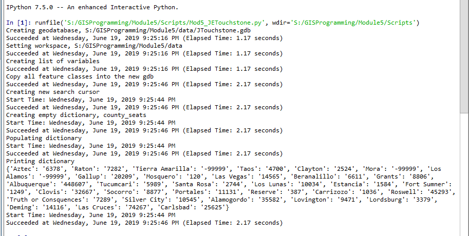
Module 5 - Manipulating Data

Well, this had to of been the toughest week for me so far. The resources that we have such as ESRI Help and the articles given to us, it is pretty straightforward gathering the proper code instructions to run the processes at hand. The thing that held me back were syntax errors, hundreds of syntax errors. There was a portion of the script that I simply just had to work around and print the info manually, I attempted everything I knew how to do and just couldn't get it to run properly. I would really like to see a script that was written for the objective and analyze it to see what I did that was incorrect. 

Module 4 - Geoprocessing

 This week we worked on geoprocessing. We also touched base on one of my favorite features and tools to utilize when creating a script for python. We used the model builder that is built in to ArcGIS Pro. The function essentially works the same as it did in ArcMap minus a few benefits, such as transposing the model to a script. Nevertheless, the model builder allows you to visualize what you are doing and the flow to approach your problem with. We used the model builder alter a feature in ArcPRO. We used the basin shapefile and clipped out the non suitable soils. We then created a script where we created an xy coordinate for a feature, a buffer, and then finally dissolved buffers.

This is a screenshot of the product of running my model builder.

This is a screenshot of my script after being ran.

Round 2- Programming Module 1

   This week was pretty straight forward. We were to implement a pre-written script in order to import the folders that will be used for this course. I was introduced to Spyder, which I had not previously used before. This will be my second time taking programming, I took it as an undergraduate core class in order to obtain my minor in GIS. I am not a grad student in the GIS Administration program and will be taking it again. I hope to retain a ton of knowledge this time around since I already have a foundation in the concepts.

Proportional & Bivariate Symbol Mapping

This lab focused on the use of proportional symbol maps and bivariate symbol mapping. The first map below is a map of the populations of the largest cities in India. I used proportional symbols to represent different values of the population fields for each of these cities. 3 classes were used to symbolize this information, 5 classes is what I was originally working with but it turned out to be too busy and quite difficult to construct the legend properly with more than 3 symbols. To create the stacked legend here, I just inserted a normal legend then converted it to graphics. From here I ungrouped the elements then proceeded to piece them together into what you see in the map below. The colors were chosed intentionlally to assist in legibility of the map. The countries surrounding India, the water feature, and the land mass of India were all symbolized with unsaturated colors. The symbols were then done with an overly saturated red color and outlined with a light red/yellow to help the smaller symbols stand out easier. 

Below is a nother proportionaly symbol map but there are two seperate fields, increase and decrease in jobs. The legend was pieced together to symbolized both of these fields. The difficult part was allowing all the symbols to be visibile, this was done by rearranging the drawing order and transparency to ensure all symbols could be seen. 

In order to create the map below I took each of the variables data and set them up into a quantile classification system with 3 classes. From here I recorder the class breaks. Using select by attribute, I chose the grouping of the first class break, second, and third for each group giving them 1,2, or 3 as their names, then A, B, or C for the next group. From here I created a unique values symbology classification with the 9 possible outcomes and inserted the legend. I converted that legend to graphics and manually manipulated the legend into the bivariate legend you see below. 

Analytical Data - Obesity and its Relationship with Poor Health

This weeks lab assignment consisted of finding some positive relationships between at least 2 variables in the county health rankings national data, from 2015. I chose to dissect the relationship between adult obesity and reported poor health. I chose a color scheme of pink and orange and worked on creating the entire map(infographic) the same theme. With the two state boundary maps I represented the percentages of these variables with the use of a graduated color scheme from lightest being the least percent and darkest being the most. Just by looking at these two examples the viewer can begin to piece together the relationships of areas where there is a correlation between the two. I chose to use bar graphs to represent the top and bottom three percent of each of the variables, and use their respective color schemes to help represent them and stay with the overall theme of the infographic. I created a graphic representation of the changes in obesity from the 70s to now by using a graphic that was downloaded and edited to represent said data and make it appear seamless and intentional. I used the scatter plot correlation data as well, to help better understand the relationship between the two as well as the mixed variable bar and line chart on the center bottom. With this chart you can see the increase in obesity with the increase in reported poor health. The chart almost makes the data appear a little less significant though, in my opinion. Then on the right side of the page I have a circle graph representing the number of people in the nation who report poor health as well as some facts about disease, health, and obesity. I am very happy with how this infographic turned out!